The comparison of algorithms is an active area of work. When we start learning algorithms, or more advanced programming, we learn of different ways of doing the same complex task. The most usual first example is sorting, which introduces a series of different ways to sort a single array, such as selection sort, insertion sort, quick sort, merge sort, etc. When comparing these algorithms, we take into account a few things: how fast it is, how much memory it needs, what are the best/worst/average-case complexities, and so on.
However, in some areas, specially applied mathematics, we have an added complication: does the algorithm work? (Or does it work with a given budget?) That happens because some types of problems don’t have an algorithm that can solve every problem. In particular, consider the problem of finding the minimum value of a function $f:\mathbb{R}^n\rightarrow\mathbb{R}$ on a set $\Omega \subset \mathbb{R}^n$. There are no algorithms that solve this problem for any given $f$ and $\Omega$, and even for specific, easier, cases, such as when $f$ is twice-continuously differentiable and $\Omega = \mathbb{R}^n$, it could happen that the algorithm steps would take more time than allowed (or some other budget contraint). In these cases, we need another type of comparison between algorithms that take into account the number of problems that are solved.
Performance Profile
Described by Dolan and Moré [1] –
(Edit: 08/08/2022) Professor André L. Tits brought to my attention the 1996 paper by Tits and Yang [3] that was already doing a profile comparison using a cumulative distribution of relative time.
– the performance profile takes into account the number of problems solved as well as the cost it took to solve it. It scaled the cost of solving the problem according to the best solver for that problem. Given a set of problems $P$ and a set of algorithms $S$, we define $c _ {s,p}$ as the cost of solving problem $p \in P$ by algorithm $s \in S$. If algorithm can’t solve the problem $p$, we define $c _ {s,p} = +\infty$. We assume that at least one algorithm solves problem $p$. The best algorithm for a given problem is the one that solves it with the least cost, i.e., we define
$$ c _ {\min,p} = \min _ {s\in S} c _ {s,p}. $$
Now we define the relative cost of the algorithm on a problem:
$$ r _ {s,p} = \frac{ c _ {s,p} }{ c _ {\min,p} }. $$
Notice that $r _ {s,p} \geq 1$, with $r _ {s,p} = 1$ meaning that algorithm $s$ is (one of) the best for problem $p$. Finally, the performance function of algorithm $s$ is given by
$$ P*s(t) = \frac{ |\{p \in P \mid\ r * {s,p} \leq t\}| }{ |P| }. $$
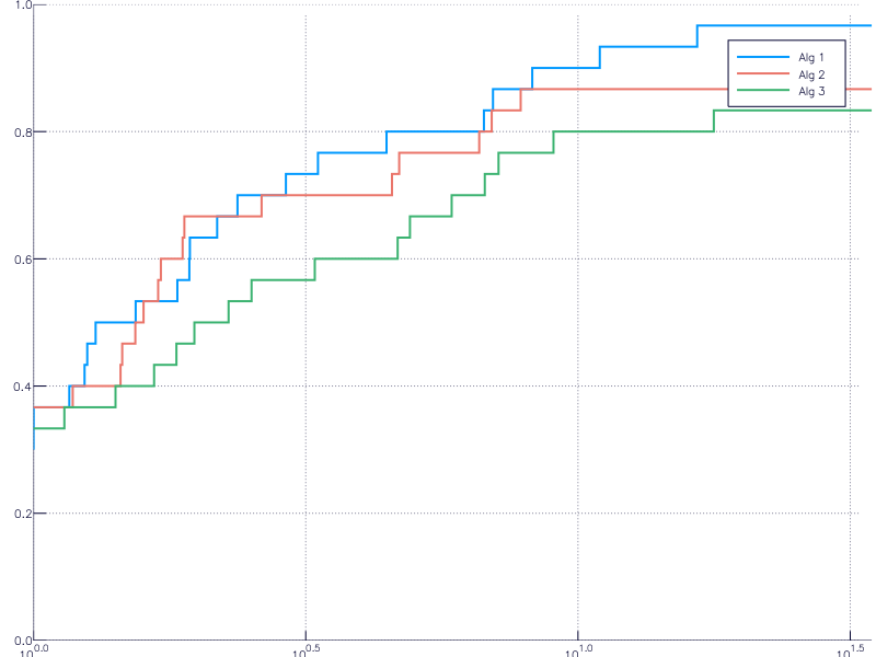
See that $P_s(1)$ is the number of problems such that $r _ {s,p} = 1$, that is the number of problems for which algorithm $s$ is one of the best. Furthermore, $P_s(r _ {\max})$ is the number of problems solved by algorithm $s$, where
$$r _ {\max} = \max _ {s \in S,\ p \in P} r _ {s,p}. $$
The value $P_s(1)$ is called the efficiency of algorithm $s$ and $P_s(r _ {\max})$ is the robustness.
The following image shows an example of performance profile:
 .
.
Example
I’m gonna create a simple example. Suppose there are 30 problems and 3 solvers and the the following matrix stores the values of $c _ {s,p}$:
c = rand(30, 3)
c[rand(1:90, 10)] = Inf # To simulate failure
The following code computes the minimum, the ratios and the performance function plots:
cmin = minimum(c, 2)
R = c ./ cmin
t = sort(unique(R))
if t[end] == Inf
  pop!(t)
end
plot(xaxis=:log)
for i = 1:size(c, 2)
  plot!(t, [sum(R[:,i] .<= ti)/size(c,1) for ti in t], label="Alg $i", t=:steppre, lw=2)
end
ylims!(0, 1)
The resulting image is
 .
.
Implementations
The traditional implementation of the performance profile was in MatLab, but I can’t find it now. Let me know if you have a link to it, so I’ll add here.
Another implementation was made by me, Raniere Gaia, and Luiz-Rafael Santos [2], in Python, but works as an external program too. We haven’t updated it in a while. Contact me if you’re interested in helping. Here’s the link.
Last, but not least, there is an implementation in Julia made by Dominique Orban, which is part of the JuliaSmoothOptimizers organization. The direct link is here.
References
[1] Elizabeth D. Dolan and Jorge J. Moré. Benchmarking optimization software with performance profiles. Mathematical Programming, 91(2):201-213, 2002. DOI: 10.1007/s101070100263.
[2] A. S. Siqueira, R. G. Costa da Silva, and L.-R. Santos. Perprof-py: A Python Package for Performance Profile of Mathematical Optimization Software. Journal of Open Research Software, 4(1), p.e12, 2016. DOI: 10.5334/jors.81.
[3] A.L. Tits and Y. Yang. Globally convergent algorithms for robust pole placement by state feedback. IEEE Transactions on Automatic Control, 41(10):1432-1452, 1996. DOI: 10.1109/9.539425.