Interoperability
Julia can natively call C and Fortran functions, and with the help of packages it can also access code from other languages, such as Python and R.
Julia has a "no boilerplate" philosophy for C and Fortran code. There's no "glue" code, code generation of compilation. To exemplify this, let's consider two files, one in Fortran and one in C:
! File lu_fact.f90
subroutine lu_factorization (nrow, ncol, A)

  implicit none

  integer, intent(in) :: nrow, ncol
  real, intent(inout), dimension(nrow, ncol) :: A

  integer :: i, j, k

  do j = 1,nrow
    do i = j+1,nrow
      A(i,j) = A(i,j) / A(j,j)
      do k = j+1,ncol
        A(i,k) = A(i,k) - A(j,k) * A(i,j)
      enddo
    enddo
  enddo

end
The code above implements the LU factorization, without pivoting or checks. The input matrix is also used as output. The factorization is used to solve linear systems.
The code below implements the forward and back substitutions, using the resulting matrix from above as input. The input vector x corresponds to the right-hand side vector on input, and as the solution of the linear system on output.
// File lu_solve.c
#include <stdio.h>

void lu_solve(long long n, float *LU, float *x)
{
  int i, j;

  for (i = 0; i < n; i++)
    for (j = 0; j < i; j++)
      x[i] -= LU[i + j * n] * x[j];

  for (i = n - 1; i >= 0; i--)
  {
    for (j = i + 1; j < n; j++)
      x[i] -= LU[i + j * n] * x[j];
    x[i] /= LU[i + i * n];
  }
}
The file lu_fact.f90 is in Fortran 90 and lu_solve.c is in C, as the extension implies. To compile these file to use with Julia, we have to prepare them into a shared library. To that end, we'll compile them using the GCC/GFortran compilers with the -fPIC -shared flags, and then link them with ld.
The following commands were tested on linux:
gfortran -fPIC -shared lu_fact.f90 -o lu_fact.o
gcc -fPIC -shared lu_solve.c -o lu_solve.o
ld -shared $PWD/lu_fact.o $PWD/lu_solve.o -o lu.so
The $PWD variable is necessary because the shared library should know where the compiled packages are. There are other ways of doing this.
Now we can use the library lu.so on Julia. Here's an example:
using Libdl, LinearAlgebra

path = "assets/interoperability"
lib = joinpath(path, "lu.so")

n = 10
L = tril(rand(Float32, n, n), -1) + I
U = triu(rand(Float32, n, n))
A = L * U
b = A * ones(Float32, n)

LU = copy(A)
x = copy(b)

ccall(
  (:lu_factorization_, lib),
  Cvoid,
  (Ref{Int}, Ref{Int}, Ref{Cfloat}),
  n, n, LU,
)

ccall(
  (:lu_solve, lib),
  Cvoid,
  (Int, Ref{Cfloat}, Ref{Cfloat}),
  n, LU, x,
)

println("‖LU - (L + U - I)‖ = ", norm(LU - L - U + I))
println("‖x - 1‖ = ", norm(x .- 1))
println("‖A * x - b‖ = ", norm(A * x - b))
‖LU - (L + U - I)‖ = 2.414704e-6
‖x - 1‖ = 2.3439863e-5
‖A * x - b‖ = 2.3841858e-6
The first part of the code defines a "good" matrix A and b such that the solution to the linear system is x = ones(n). The LU = copy(A) and x = copy(b) are so that we can use A and b for testing later. One important part of the code is that since we used the default variables for Fortran, we used float for C, and we have to use an appropriate type for Julia as well. Float32 refers to a 32 bits real number, i.e. float. Cfloat is just an alias for Float32.
The ccall signature is simple:
The first argument is the function or a tuple with the function and it's library;
The second argument is the return type;
The third argument is a tuple with the types of every argument;
The other arguments are the arguments to the C/Fortran function.
Noteworthy:
Fortran with
gfortranadded a_to the function name;Ref{T}indicates that a reference will be passed, allowing the argument to be modified (Ptr{T}also exists, to indicate returned pointers by C);Fortran always passes variables by reference.
FFTW
For a more substantial example, we can look at the FFTW Library for the discrete Fourier transform. The compilation of this example takes some time and the installation may be less straightforward than in my system, so be warned.
First, download the library. I'm using v3.3.10. Untar it too.
Then, enter the folder and issue a
./configure --enable-shared.Now, enter
make.
This will produce a shared library .libs/libfftw3.so.
Now we can write a function to compute the FFT of a given vector using this lib.
We'll be create a simple version of the following C code, available in the online docs of FFTW.
#include <fftw3.h>
...
{
    fftw_complex *in, *out;
    fftw_plan p;
    ...
    in = (fftw_complex*) fftw_malloc(sizeof(fftw_complex) * N);
    out = (fftw_complex*) fftw_malloc(sizeof(fftw_complex) * N);
    p = fftw_plan_dft_1d(N, in, out, FFTW_FORWARD, FFTW_ESTIMATE);
    ...
    fftw_execute(p); /* repeat as needed */
    ...
    fftw_destroy_plan(p);
    fftw_free(in); fftw_free(out);
}
function myfft(x::Vector{ComplexF64})
y = copy(x)
FFTW_FORWARD = Int32(-1)
FFTW_ESTIMATE = Int32(64)
plan = ccall(
(:fftw_plan_dft_1d, "assets/interoperability/fftw-3.3.10/.libs/libfftw3.so"),
Ptr{Cvoid},
(Int32, Ref{ComplexF64}, Ref{ComplexF64}, Int32, UInt32),
length(x), x, y, FFTW_FORWARD, FFTW_ESTIMATE
)
ccall(
(:fftw_execute, "assets/interoperability/fftw-3.3.10/.libs/libfftw3.so"),
Cvoid,
(Ptr{Cvoid},),
plan
)
ccall(
(:fftw_destroy_plan, "assets/interoperability/fftw-3.3.10/.libs/libfftw3.so"),
Cvoid,
(Ptr{Cvoid},),
plan
)
return y
end
x = rand(ComplexF64, 8)
y = myfft(x)8-element Vector{ComplexF64}:
4.8563398366457 + 4.918043077845817im
-0.5584713687872389 - 0.06972589172145907im
1.1595202486828367 - 0.39028854391493795im
-0.9715037230022334 - 1.9489890967053087im
0.564273701601059 + 0.2184975837835994im
0.19601917302905525 + 0.09751647349067052im
-0.6983040806953942 - 0.5176872658813294im
1.0159206572089095 - 0.8465624562760898imWe can implement the a basic DFT to compare:
function mydft(x)
  n = length(x)
  return [
    sum(x[i+1] * exp(-im * 2π * i * k / n) for i = 0:n-1)
    for k = 0:n-1
  ]
end
mydft(x)
8-element Vector{ComplexF64}:
4.8563398366457 + 4.918043077845816im
-0.5584713687872391 - 0.06972589172145949im
1.1595202486828364 - 0.39028854391493806im
-0.9715037230022335 - 1.948989096705309im
0.5642737016010596 + 0.21849758378359918im
0.19601917302905442 + 0.09751647349066861im
-0.6983040806953944 - 0.5176872658813332im
1.0159206572089108 - 0.8465624562760865imYou may have noticed:
Memory is handled by Julia in this case, so we don't use
malloc.The C struct
fftw_complexsimply stores twodoubles. In Julia we would need a similar struct, andComplexF64is exactly that, so it's extra smooth.We can use
Ptr{Cvoid}to avoid dealing with the return type offftw_plan_dft_1d, which is an opaque pointer.
FFTW.jl (and where are the .so files?)
The ability to easily integrate C/Fortran functions is also one of the foundations of Julia. In fact, the example above is adapted from a 2011 commit almost unmodified. The FFTW package is now wrapped in the package FFTW.jl. You can add and use it easily:
using FFTW
y = fft(x)
8-element Vector{ComplexF64}:
4.8563398366457 + 4.918043077845817im
-0.5584713687872389 - 0.0697258917214591im
1.1595202486828367 - 0.39028854391493795im
-0.9715037230022334 - 1.9489890967053087im
0.564273701601059 + 0.2184975837835994im
0.1960191730290552 + 0.0975164734906705im
-0.6983040806953942 - 0.5176872658813294im
1.0159206572089095 - 0.8465624562760898imIf you install FFTW.jl, you will notice that you don't need to install the C library FFTW manually, i.e., the Julia package automatically does that for you. Julia has a built-in Artifacts system and a commonly used package BinaryBuilder.jl that work in conjunction to allow binaries to be pre-built and distributed. The details are complicated, but the user doesn't have to worry about them.
Python
Julia can also can Python and R code, using PyCall and RCall, respectively. We'll focus on Python for this example.
We're gonna use PyCall. Like IJulia,
using Plots, PyCall, Random
pyplot()

Random.seed!(123)
n = 2^8
X = (2 * rand(n, 2) .- 1) * 4
y = [
  X[i,2]^2 * 16 - X[i,1]^2 * 16 ≤ 2 * randn() ? 1 : -1 for i = 1:n
]
y = [
  (X[i,1] - 1)^2 + (4 - randn()) * (X[i,2] - X[i,1]^2)^2 ≤ 10 ? 1 : -1 for i = 1:n
]
plot(leg=false)
idx = findall(y .== -1)
scatter!(X[idx,1], X[idx,2], m=(4,:red,:square))
idx = findall(y .== 1)
scatter!(X[idx,1], X[idx,2], m=(4,:blue,:circle))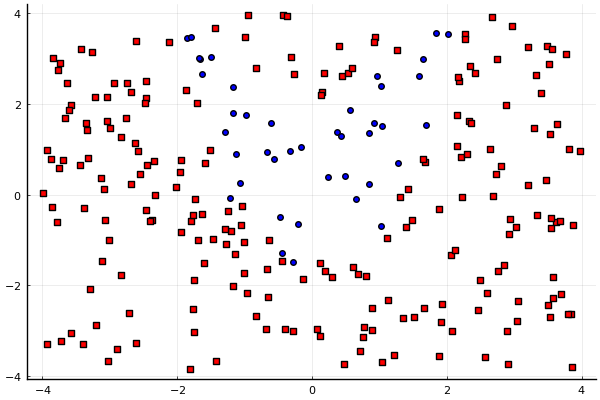
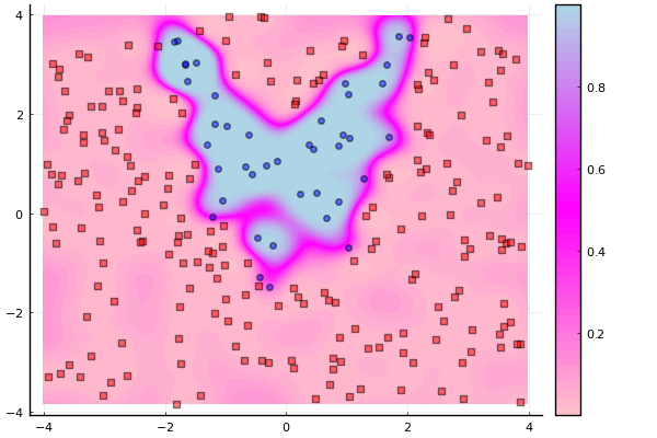
svm = pyimport_conda("sklearn.svm", "scikit-learn")
clf = svm.SVC(C=1e-2, gamma=5.0, probability=true)
clf.fit(X, y)
x1g = range(extrema(X[:,1])..., length=100)
x2g = range(extrema(X[:,2])..., length=100)
Z = [
  clf.predict_proba([x1i x2j;])[2] for x2j in x2g, x1i in x1g
]
contourf(x1g, x2g, Z, c=cgrad([:pink,:magenta,:lightblue]), levels=50)
idx = findall(y .== -1)
scatter!(X[idx,1], X[idx,2], m=(4,:red,:square), lab="", opacity=0.5)
idx = findall(y .== 1)
scatter!(X[idx,1], X[idx,2], m=(4,:blue,:circle), lab="", opacity=0.5)