Parallel

Parallelization is hard and is not my specialty, so I'll focus on a simple example. See more here.

Atention: Before we start, you should either:

Set "Julia: Num Threads" in your VSCode to the number of threads that you can use; or
Pass the number of threads to the julia call: julia --threads N.

Check the number of threads being used with

Threads.nthreads()

We'll compute the approximate value of $\pi$ using Monte Carlo simulation. This example is based on Parallel Programming in Python.

The idea is pretty simple, and you might have seen it before. Consider a square with vertices $(0,0)$ , $(1,0)$ , $(0,1)$ and $(1,1)$ , and the sector of the circle centered at $(0,0)$ with radius $1$ .

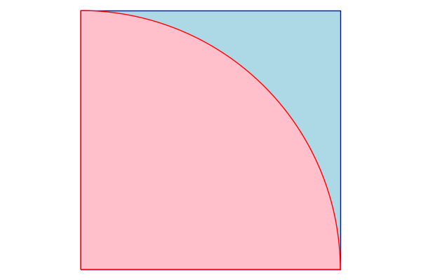
The square's area is $1$ , and the circle's area is $\pi / 4$ . The ratio being $\pi / 4$ , then.

The Monte Carlo approach is to generate a number $N$ os points equally distributed on the square. Let $M$ be the number of points that fall inside the sector. The ratio $M / N$ should assintotically approach the ratio $\pi / 4$ , therefore an approximation to $\pi$ can be obtained by computing $4M / N$ .

Here's a basic implementation:

function calc_pi(N)
  M = 0
  for i = 1:N
    x, y = rand(), rand()
    if x^2 + y^2 < 1
      M += 1
    end
  end
  return 4 * M / N
end

calc_pi (generic function with 1 method)

Here are some histogram of the error using various $N$ various for 100 simulations each:

N_values = 10 .^ (5:7)
plt = plot(layout=grid(3, 1), size=(400,600), leg=false)
for (i, N) in enumerate(N_values)
  ϵ = π .- [calc_pi(N) for _ = 1:200]
  histogram!(plt[i], ϵ, bins=20)
  title!(plt[i], "N = $N")
end
plt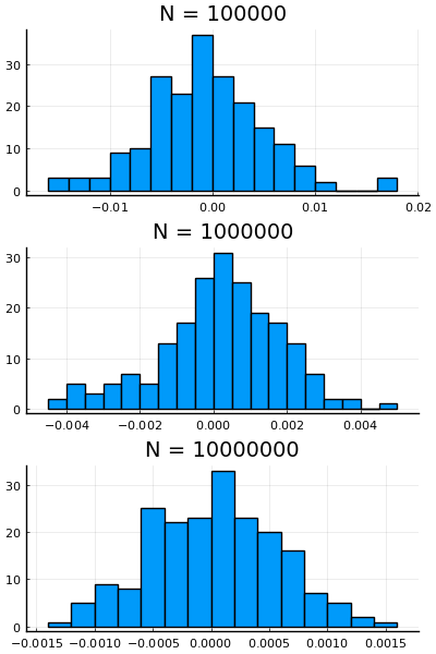

Using @time we can assess the computation time of calc_pi:

@time calc_pi(10^7)

  0.105775 seconds
3.1424504

Be aware that Julia compiles the code as it is first executed. In this case, since we ran the code before, the timing is mostly accurate.

That being said, measuring execution time of code has some randomness, so it's better to run the code a few times and compute some statistics (mean, median, minimum, maximum, etc.) on the result. Luckily, the package BenchmarkTools does that for us.

You can use @btime "Your stuff" to compute the equivalent of @time, but we can see more information with @benchmark:

using BenchmarkTools

println("π ≈ $(calc_pi(10^7))")
@benchmark calc_pi(10^7)

π ≈ 3.1417864
BenchmarkTools.Trial: 46 samples with 1 evaluation.
 Range (min … max):  103.256 ms … 117.549 ms  ┊ GC (min … max): 0.00% … 0.00%
 Time  (median):     108.468 ms               ┊ GC (median):    0.00%
 Time  (mean ± σ):   108.740 ms ±   2.890 ms  ┊ GC (mean ± σ):  0.00% ± 0.00%

  ▁             ▁  ▄ ▁ ▄▁▁▄▁  ▁█                                 
  █▁▁▁▁▁▆▆▆▁▆▆▆▆█▆▆█▁█▆█████▁▁██▆▁▆▆▁▁▆▁▁▁▆▁▆▁▁▆▁▁▁▁▁▆▁▁▁▁▁▁▁▁▆ ▁
  103 ms           Histogram: frequency by time          118 ms <

 Memory estimate: 0 bytes, allocs estimate: 0.

Unlike Python, vectorizing the code won't improve the performance:

function calc_pi_vectorized(N)
  pts = rand(N, 2)
  M = count(sum(pts .^ 2, dims=2) .< 1)
  return 4 * M / N
end

println("π ≈ $(calc_pi_vectorized(10^7))")
@benchmark calc_pi_vectorized(10^7)

π ≈ 3.1410816
BenchmarkTools.Trial: 23 samples with 1 evaluation.
 Range (min … max):  197.942 ms … 467.868 ms  ┊ GC (min … max):  2.78% … 58.74%
 Time  (median):     204.382 ms               ┊ GC (median):     4.27%
 Time  (mean ± σ):   223.463 ms ±  66.903 ms  ┊ GC (mean ± σ):  12.32% ± 14.69%

  ██                                                             
  ██▅▄▁▁▁▁▁▁▁▁▁▁▁▁▁▁▁▁▁▁▁▁▁▁▁▁▁▁▁▁▁▁▁▁▁▁▁▁▁▁▁▁▁▄▁▁▁▁▁▁▁▁▁▁▁▁▁▁▄ ▁
  198 ms           Histogram: frequency by time          468 ms <

 Memory estimate: 382.67 MiB, allocs estimate: 14.

We can, however, use threads to improve it. The code below has a few simple changes to have an improved version.

using Base.Threads: @threads, threadid, nthreads

function calc_pi_threaded_naive(N)
  M = zeros(Int, nthreads())
  @threads for i = 1:N
    x, y = rand(), rand()
    if x^2 + y^2 < 1
      M[threadid()] += 1
    end
  end
  return 4 * sum(M) / N
end

println("π ≈ $(calc_pi_threaded_naive(10^7))")
@benchmark calc_pi_threaded_naive(10^7)

π ≈ 3.141158
BenchmarkTools.Trial: 32 samples with 1 evaluation.
 Range (min … max):  149.629 ms … 172.437 ms  ┊ GC (min … max): 0.00% … 0.00%
 Time  (median):     155.640 ms               ┊ GC (median):    0.00%
 Time  (mean ± σ):   156.825 ms ±   5.078 ms  ┊ GC (mean ± σ):  0.00% ± 0.00%

           ██  ▃   █  ▃   ▃        ▃                             
  ▇▇▁▁▇▁▇▁▇██▇▁█▇▇▁█▁▇█▁▁▁█▁▇▇▁▁▁▁▇█▁▇▁▁▁▁▁▁▁▁▁▁▁▁▁▁▁▁▇▁▁▁▁▁▁▁▇ ▁
  150 ms           Histogram: frequency by time          172 ms <

 Memory estimate: 640 bytes, allocs estimate: 7.

The version above creates the a vector to store the number of points inside the circle per thread. We could be more naive and use a single M, but for sharing between threads, M must be an array.

This version simply uses the Base.Threads module in the form of the macro @threads before the for. The macro splits the for between the threads automatically.

As you saw, though, the result is slower than the basic version. To fix this, we have to use thread-safe random number generators. The code below does this and improves the execution time in comparison to the original.

using Random

function calc_pi_threaded(N)
  M = zeros(Int, nthreads())
  @threads for i = 1:N
    rng = Random.THREAD_RNGs[threadid()]
    x, y = rand(rng), rand(rng)
    if x^2 + y^2 < 1
      M[threadid()] += 1
    end
  end
  return 4 * sum(M) / N
end

println("π ≈ $(calc_pi_threaded(10^7))")
@benchmark calc_pi_threaded(10^7)

π ≈ 3.1411528
BenchmarkTools.Trial: 52 samples with 1 evaluation.
 Range (min … max):  93.523 ms … 106.825 ms  ┊ GC (min … max): 0.00% … 0.00%
 Time  (median):     97.610 ms               ┊ GC (median):    0.00%
 Time  (mean ± σ):   98.051 ms ±   2.720 ms  ┊ GC (mean ± σ):  0.00% ± 0.00%

  ▁          ▁▄ ▁▁ ▁█▁▁▄▁▁▁  ▁  ▄  ▁    ▁                       
  █▁▁▁▆▆▆▆▁▆▁██▆██▁████████▁▆█▁▁█▁▆█▁▆▁▁█▁▁▁▁▁▁▁▁▆▁▁▁▆▁▁▁▁▁▁▁▆ ▁
  93.5 ms         Histogram: frequency by time          106 ms <

 Memory estimate: 640 bytes, allocs estimate: 7.

But wait, there's more. We can manually split the range, and just use @threads over the ranges.

using Distributed: splitrange

function calc_pi_proper_threaded(N)
  ranges = splitrange(1, N, nthreads())
  M = Ref(0)
  @threads for rg in ranges
    rng = MersenneTwister()
    c = 0
    for _ in rg
      c += rand(rng)^2 + rand(rng)^2 < 1
    end
    M[] += c
  end
  return 4 * M[] / N
end

println("π ≈ $(calc_pi_proper_threaded(10^7))")
@benchmark calc_pi_proper_threaded(10^7)

π ≈ 3.1417084
BenchmarkTools.Trial: 123 samples with 1 evaluation.
 Range (min … max):  38.890 ms … 47.793 ms  ┊ GC (min … max): 0.00% … 0.00%
 Time  (median):     40.399 ms              ┊ GC (median):    0.00%
 Time  (mean ± σ):   40.846 ms ±  1.418 ms  ┊ GC (mean ± σ):  0.00% ± 0.00%

         ▃██ ▄      ▂                                          
  ▃▁▁▆▆▃▇███████▇▆▇██▅▅█▆▆▃▅▁▅▅▃▃▃▁▁▃▁▃▃▃▁▁▁▃▁▃▃▁▁▁▁▃▃▁▁▃▁▁▁▃ ▃
  38.9 ms         Histogram: frequency by time        45.6 ms <

 Memory estimate: 20.20 KiB, allocs estimate: 19.

We use Ref(0) now to keep a reference to a number that all threads can access.

Finally, we can use the package FLoops and change very little to obtain still some more speed. I don't know why, though.

using FLoops

function calc_pi_proper_floop(N)
  ranges = splitrange(1, N, nthreads())
  @floop for rg in ranges
    rng = MersenneTwister()
    c = 0
    for _ in rg
      c += rand(rng)^2 + rand(rng)^2 < 1
    end
    @reduce(M += c)
  end
  return 4 * M / N
end

println("π ≈ $(calc_pi_proper_floop(10^7))")
@benchmark calc_pi_proper_floop(10^7)

π ≈ 3.1412868
BenchmarkTools.Trial: 125 samples with 1 evaluation.
 Range (min … max):  38.244 ms … 46.224 ms  ┊ GC (min … max): 0.00% … 0.00%
 Time  (median):     39.706 ms              ┊ GC (median):    0.00%
 Time  (mean ± σ):   40.073 ms ±  1.403 ms  ┊ GC (mean ± σ):  0.00% ± 0.00%

       ▃▅█▅▂▅▄    ▂                                            
  ▅▃▇█▇███████▆▆▆▃█▃██▅▆▁▅▅▇▃▁▁▁▅▅▁▁▁▃▁▁▁▁▁▁▃▁▁▁▁▁▁▁▃▁▁▁▁▁▁▁▃ ▃
  38.2 ms         Histogram: frequency by time        46.2 ms <

 Memory estimate: 19.78 KiB, allocs estimate: 19.