Creating a package: SequGen.jl - demonstration of good practices
In this section we'll look into implementing and registering a package, following some good practices.
What is/will be SequGen
SequGen.jl will be a package to implement time series/sequences generation on Julia. It is based on the homonymous NLeSC project sequgen.
In this tutorial, our package will generate simple time series that we'll be able to add up and create useful synthetic data. We'll work with structs and showcase multiple dispatch in the process.
Create the package skeleton
Not much is needed to create a proper package in Julia. It needs to follow a basic structure of the form
PackageName.jl
- src/
  - PackageName.jl
- test/
  - runtests.jl
- Project.toml
The entry point of the package is the src/PackageName.jl file. The test/runtests.jl file is run when you try to pkg> test a package. Finally, the Project.toml file contains several information about the package:
name: Nameuuid: A unique identifierauthors: A list of authorsversion: A SemVer version.[deps]: A list of packages and their UUIDs.[compat]: A list of packages and the versions needed for this package.[extras]: A list of additional packages used for testing.[targets]: Additional targets (and their required packages). Currently only supportstestfor the testing packages.
An easy way to generate a basic skeleton for pacakges is using the built-in pkg> generate PackageName. However, since we usually want a bunch of other goodies, we can use the package PkgTemplates instead.
First, pkg> add PkgTemplates and julia> using PkgTemplates. Then simply run
julia> generate("SequGen")Template keywords to customize:
[press: d=done, a=all, n=none]
[ ] user
[ ] authors
[ ] dir
[ ] host
[ ] julia
[ ] pluginsA list of options will appear to allow customization. Fow now, select dir and plugins.
Template keywords to customize:
[press: d=done, a=all, n=none]
   [ ] user
   [ ] authors
   [x] dir
   [ ] host
   [x] julia
 > [x] plugins
Press d
Enter value for 'dir' (String, default="~/.julia/dev"):The first option, dir, allows us to choose where to save our package. Julia's default dev environment is inside .julia/dev/ in the home folder. To avoid having to look for it, simply enter . (a single dot).
The next options selects the minimum Julia version that our package will support.
Select minimum Julia version:
   1.0
   1.1
   1.2
   1.3
   1.4
   1.5
 > 1.6
   Other
Some notes:
Version 1.0 is the first stable version, but the next versions add some extra goodies, as well as being more efficient.
Version 1.3 is the first version with a lot of new important features, and it's frequently preferred over 1.0.
Version 1.6 is, at the time of writing, chosen as the next Long Term Support (LTS) version. That change will take effect as soon as 1.7 is released.
Version 1.7 is, at the time of writing, on the verge of being released. Hopefully it should be released by time this workshop takes place.
We'll select 1.6, assuming it is the LTS version.
The
Select plugins:
[press: d=done, a=all, n=none]
   [X] CompatHelper
   [X] ProjectFile
   [X] SrcDir
   [X] Git
   [X] License
   [X] Readme
   [X] Tests
   [X] TagBot
 > [ ] AppVeyor
   [ ] BlueStyleBadge
   [ ] CirrusCI
   [ ] Citation
   [ ] Codecov
   [ ] ColPracBadge
   [ ] Coveralls
   [ ] Develop
   [ ] Documenter
   [ ] DroneCI
   [ ] GitHubActions
   [ ] GitLabCI
   [ ] RegisterAction
   [ ] TravisCI
The second option gives as a wide range of plugins, many of which we want. In addition to the ones that are already selected, choose Citation, Codecov, Documenter, GitHubActions and RegisterAction. Their meaning are as follows:
Citation: Creates aCITATION.bibfile for citing package repositories.CompatHelper: Integrates your packages with CompatHelper via GitHub Actions. This automatically checks for updates on the dependencies and creates a pull request updating the version bounds.Codecov: Sets up code coverage submission from CI to Codecov.Documenter: Sets up documentation generation via Documenter.jl. The deploy depends on a CI, and in this case we're choosing GitHub Actions.Git: Creates a Git repository and a.gitignorefile.GitHubActions: Integrates your packages with GitHub Actions. Currently the most used CI for Julia packages after Travis CI support for open source software went downhill.License: Creates a license file (defaults to using MIT).ProjectFile: Creates a defaultProject.toml.Readme: Creates aREADMEfile that contains badges for other included plugins.RegisterAction: Add a GitHub Actions workflow for registering a package with the General registry via workflow dispatch. See here for more information.SrcDir: Creates a module entrypoint.TagBot: Adds GitHub release support via TagBot. This automatically creates a git tag and a GitHub release.Tests: Sets up testing for packages.
After selecting these, simply accept the default options for the plugins using d.
Warning: When the process arrives at Documenter, you'll need to select how to deploy the documentation. We're using GitHub Actions, so select that.
The current default (2021-09-23) leaves us with the following structure:
.github/
workflows/
CI.yml
CompatHelper.yml
register.yml
TagBot.yml
docs
src
index.md
make.jl
Manifest.toml
Project.toml
src
PackageName.jl
test
runtests.jl
.gitignore
CITATION.bib
LICENSE
Manifest.toml
Project.toml
README.md
A .git folder is also present, but we'll ignore it.
Some information about Project and Manifest
Julia has a built-in package manager: Pkg. When you press ] on the REPL, it turns into pkg> to indicate that pkg mode is on. From there, you can add packages, like we did above, but also remove, change versions, instantiate, etc.
A Project.toml file defines an environment, which can be a package or not, in which specific packages are installed. The package fields [deps] describes which packages are/should be installed in the environment, and [compat] can show which versions of the packages are allowed. In other words, Project.toml provides the requirements of our environment.
The Project.toml file indicate the required packages and their supported versions. When you install the packages, the actual installed versions are kept on the file Manifest.toml. That means that with Manifest.toml, you can recreate the exact Julia's environment using pkg> instantiate.
Project.toml and Manifest.toml work together. Project.toml is for humans, and Manifest.toml is only useful for humans when we want exact control of the environment situation. For instance, Project.toml may define that we need SomePackage version 1.6. If a small bugfix is released for SomePackage, we'll probably want to accept it in our project, i.e., we want version 1.6.1. However, we don't want to constrain the version to 1.6.1, because we don't actually need it. Furthermore it would be counter-productive to update to each individual version.
As a second example, unless SomePackage 1.7 breaks our package, we can accept version 1.7 without removing support for 1.6. That means that Project.toml will have the information that SomePackage could be 1.6 or 1.7.
In both cases, after updating, Manifest.toml will only tell the installed version, which will change after we update.
Therefore, Project.toml is stored in our git repository and Manifest.toml usually isn't. For a package, Manifest.toml is never useful. For some environments, it may be useful to keep both.
Notice that if you don't have a Manifest.toml file, running pkg> instantiate will resolve the dependencies and install versions for each package.
Uploading and checking
The repo starts with a commit and the repo setup (if you have setup git). Your next steps:
Create the repo on GitHub;
git push -u origin main, and check your CI.(optional) Go to Codecov, find the repo an turn coverage ON;
First steps
The basic idea of our package will be:
We have different types of sequences;
We want to sample these sequences at different intervals or ranges.
For instance, to describe the average temperature of a city per day we might say we need:
A constant value to set the mean value;
A sine wave for the yearly oscillation;
A random noise generator.
With this description, we can ask for sample of N points in the interval starting at 60 days and ending at 120 days. If we ask for a new sample, we'll get different noise, but the rest will be the same.
In Python, we could create a base class Sequence and a method sample(interval), or sample(start, end, length). We would then implement classes Constant, SineWave, GaussianNoise deriving from Sequence as specialize the sample method for these cases.
In Julia, it won't be so different. We'll start by creating an abstract type for Sequence and the function sample.
# File src/SequGen.jl
module SequGen

export Sequence
export sample

abstract type Sequence end

function sample end

# includes will go here

end # module
Here, exporting only gives visibility to the user that uses our package. Otherwise, he would have to write SequGen.sample to specify where sample comes from.
The function sample end simply declares that the sample function exists. This line is not really necessary, but it's useful to centralize the basic API information. We'll also add docstrings to this function, instead of somewhere else.
Next, create a file constant.jl and add the line include("constant.jl") on src/SequGen.jl.
# File constant.jl
export Constant

struct Constant <: Sequence
  x
end

sample(seq::Constant, t::AbstractVector) = fill(seq.x, length(t))
Note: Don't forget to add include("constant.jl") to src/SequGen.jl.
Now, Constant is a subtype of Sequence that contains a field x of indeterminate type (Any). We also defined how the sample function behaves for a Constant and an AbstractVector: it returns a vector of size length(t) filled with seq.x.
This should already run on our REPL, so let's check.
Open a Julia REPL inside the SequGen.jl base folder.
Press
]to enterpkg>mode.Change to the general environment with
pkg> activatewithout arguments.It should read
(@v1.6) pkg>(or a newest version).pkg> add Revise, Plots, Unitful, UnitfulRecipes.Activate the current environment with
pkg> activate ..It should have changed to
(SequGen) pkg>.Return to
julia>mode by pressing the backspace.Enter
using Revise.Enter
using SequGen.Enter
s = Constant(2.3).Enter
sample(s, 1:3). It should output
3-element Vector{Float64}:
 2.3
 2.3
 2.3
Rejoice.
Now, we can add the Trend struct, to correspond to the function .
# File trend.jl
export Trend

mutable struct Trend <: Sequence
  start
  slope
end

sample(seq::Trend, t::AbstractVector) = (t .- seq.start) * seq.slope
You must
include("trend.jl")onSequGen.jl.
Notice that because of Revise, the package is reloaded and Trend is already available. So the following works.
julia> s = Trend(1.0, 0.2)
Trend(1.0, 0.2)

julia> sample(s, 1:3)
0.0:0.2:0.4

julia> sample(s, [0.0; 5.0; 10.0])
3-element Vector{Float64}:
 -0.2
  0.8
  1.8
Notice that we the function sample works differently for Constant and Trend types. This works as if we had a method sample for classes Constant and Trend in Python. What happens in Python is single dispatch, i.e., the function that is actually used when seq.sample(t) is called is dispatched on the type of seq. In Julia, we have multiple dispatch, although in the example of sample, it is only single dispatch as well. We'll see a multiple dispatch example soon.
First tests
Now, before continuing, we should add some tests. Edit test/runtests.jl as follows:
# File test/runtests.jl
using SequGen
using Test

@testset "Constant" begin
  t = 1:10
  for c in (5, 1.23)
    s = Constant(c)
    @test sample(s, t) == fill(c, 10)
  end
end

@testset "Trend" begin
  for Δt in (1, 1.0),
      t₀ in (0.0, 1.0),
      Δx in (3, 3.14)
    t = collect(range(t₀, t₀ + Δt, length=101))
    s = Trend(t₀, Δx / Δt)
    x = collect(range(zero(Δx), Δx, length=101))
    @test sample(s, t) ≈ x
  end
end
These tests simply verify that the output of sample is correct. Notice that we use ≈ (\isapprox[TAB]) to compare sample(s, t) and x, so we have to collect the ranges so they become vectors.
To test the package,
enter
pkg>(press]);pkg> test.
The test will create a separate environment and install necessary packages, if they are declared. This happens for the package Test. He is declared on Project.toml under [extras] and on the list test = ["Test"] under [targets]. Don't worry about finding out the UUID of the package. When you add it, it automatically appears on Project.toml under [deps]. you just have to, if necessary, move it to [extras].
Now it should be a good time to commit and push.
Note: At this point, you should have CI passing and 100% coverage on Codecov.
Documenting
It is also a good time to add docstrings and configure the Documenter.jl. A docstring is the information that appears when you ask for the help of a function. You can add docstrings by simply adding strings right before the function or struct definition.
We can add a docstring for sample like the following:
"Compute a sample of a given sequence on a given range."
sample(seq::Constant, t::AbstractVector) = fill(seq.x, length(t))
Now you can go to the REPL, press ? to change your REPL to help?>, and then enter sample. If Revise is loaded you should see the information you just wrote printed on the screen.
Notice that there is no signature information from the function sample. That's because this help will apply to all sample functions that are defined, even if we wildly change the signature.
The docstring is helpful already, but we can better inform the user of what's going on. Since a single line will not be sufficient, we can use multiline strings ("""...""") for the job. You should also now that the docstring is parsed as Markdown, so you can format it accordingly. The following is a better docstring:
"""
    x = sample(sequence, range)

Compute a sample of the given `sequence` in the given `range`.
"""
sample(seq::Constant, t::AbstractVector) = fill(seq.x, length(t))
By entering help?> sample again, you should see a better message, with properly colored words. Since the REPL already uses monospace fonts, the "code" bits just change in color, but the documentation that we'll produce next will properly show the difference.
In the folder docs you will see all the basic information you need to have a documentation with the package Documenter.jl, which is the Julia main package for this. The docs are themselves a different project, and as such they have a Project.toml and a Manifest.toml file. We can (and some say, should) constrain the Documenter version that will be run, or add additional packages that are not needed for our SequGen, but that would be intersting (like Plots). It is also important to know that we want to use the development version of our package, so we would need to tell the environment to use the relative package at .. (from the docs folder). The generated environment already has that setup, but keep it in mind if you have to install Documenter.jl manually.
Inside the docs folder you have a src folder, with all files that will be parsed into docs, and a make.jl file that runs the Documenter package that processes these files. The make.jl file can be a bit complicated, specially for our first usage, so I'll just point out the general idea:
makedocsis responsible for parsing thesrcfolder;pagesis a list of "pairs" declaring the page names and their corresponding sources;
deploydocsis responsible for pushing our documentation to the site, but it will only do so while running on the CI.
To run the documentation locally, we have to change folders and environments, so instead, it might be better to open another terminal on the project root and run
julia --project=docs/ -e 'include("docs/make.jl")'[ Info: SetupBuildDirectory: setting up build directory.
[ Info: Doctest: running doctests.
[ Info: ExpandTemplates: expanding markdown templates.
[ Info: CrossReferences: building cross-references.
[ Info: CheckDocument: running document checks.
[ Info: Populate: populating indices.
[ Info: RenderDocument: rendering document.
[ Info: HTMLWriter: rendering HTML pages.
┌ Warning: Documenter could not auto-detect the building environment Skipping deployment.
└ @ Documenter ~/.julia/packages/Documenter/XIxke/src/deployconfig.jl:75Don't worry about the Warning.
The folder docs/build is created. Look for index.html and open it on your browser. For instance, run
firefox docs/build/index.htmlor a different browser.
You should see something like this:
You should see a page with very little information about SequGen and our docstring for sample. To see how that appeared there, check docs/src/index.md:
# File docs/src/index.md
```@meta
CurrentModule = SequGen
```

# SequGen

Documentation for [SequGen](https://github.com/abelsiqueira/SequGen.jl).

```@index
```

```@autodocs
Modules = [SequGen]
```
The first @meta states what is the module for this file, and is overkill for many packages, since they only have a single module (as do we). Then you have a title in Markdown # SequGen and a line of information with a link for our repo. This can and should be updated to better describe the package, but not now.
The next commands are specific to Documenter.jl. Documenter uses the triple ticks with specific commands to parse our docs. The @index command generates a list of links for the docstrings. The @autodocs command looks for all docstrings in the given modules and prints them. That means that for we already have a basic documentation to start. All our documented docstrings will be printed on this single page and linked on the top. We can definitely do better, for instance creating separate pages and using @docs to explicitly tell which docstrings to print.
Putting the documentation online
Make a commit and push the changes.
The CI (you can check online what's happening and/or the CI.yml file):
Checkouts the package;
Downloads the latest
1julia;Activates the environment and includes the SequGen package in development;
Runs the doctests;
Runs the
make.jlfile.
If nothing went wrong, it should pass, and in that case you will be able to see the documentation. Go to github repo page and click on the dev badge.
When registering our package, things get a bit more convoluted. After your package is registered, the TagBot action will create a tag and release for it on GitHub to match the registered version. It will also try to build the documentation for this tagged version (stable docs). However, for security reasons, TagBot can't use the GITHUB_TOKEN secret that is readily available. Instead, you need to create a DOCUMENTER_KEY. It is better to deal with that now, to avoid headaches in the future. Feel free to skip this part, because we won't be registering our package today.
Open a REPL (or reuse) on the folder with the package;
pkg> activate(no arguments) to change the environment to home;pkg> add DocumenterToolsjulia> using DocumenterToolspkg> activate .to change the environment to SequGen;If it's a new REPL,
julia> using SequGen;julia> DocumenterTools.genkeys(SequGen)You're gonna see something like:
[ Info: add the public key below to https://github.com/abelsiqueira/SequGen.jl/settings/keys with read/write access:

ssh-rsa ONE-LINE-OF-HASH Documenter

[ Info: add a secure environment variable named 'DOCUMENTER_KEY' to https://travis-ci.com/abelsiqueira/SequGen.jl/settings (if you deploy using Travis CI) or https://github.com/abelsiqueira/SequGen.jl/settings/secrets (if you deploy using GitHub Actions) with value:

VERY-BIG-HASH
Follow the first link, add the key, mark the write access check. The name doesn't matter.
Follow the third link - we're not using Travis CI. Name the variable
DOCUMENTER_KEYand paste the full hash in there.That's it.
More sequences
Now we should have tests and documentation, so we can go back to improving our package. The next two Sequences that we'll add are the SineWave and the GaussianNoise. The sine wave is given by
where is the amplitude of the wave, is the period, and is the phase.
Therefore, we can create the following file:
# File sine-wave.jl
export SineWave

struct SineWave <: Sequence
  amplitude
  period
  phase
end

function sample(seq::SineWave, t::AbstractVector)
  return seq.amplitude * sin.(2π * t / seq.period .+ seq.phase)
end
Notice that sin. is the function sin with a dot (.), i.e., is applies the sine function all elements of the argument. Likewise with .+.
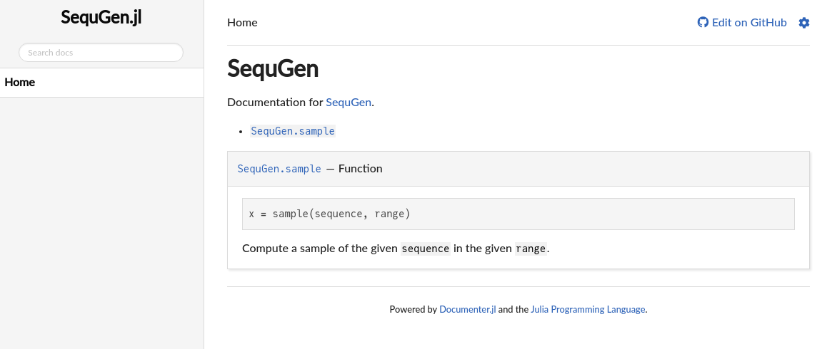
Assuming you have Plots installed, you can run the following lines in your REPL and see the result:
t = range(0, 10, length=50)
s = SineWave(2.0, 7.0, pi / 3)
y = sample(s, t)
plot(t, y)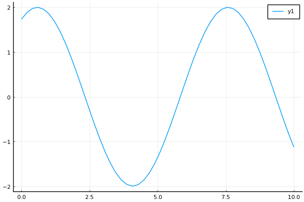
On the other hand, it would be nice to be able to create a sine wave by stating where the peak happens, instead of the phase (which is less obvious). To do that, we can create a constructor like the following:
# File sinewave .jl
# ... struct SineWave defined above
function SineWave(type::Symbol, amplitude, period, phase_or_peak)
  if type == :from_phase
    return SineWave(amplitude, period, phase_or_peak)
  elseif type == :from_peak
    phase = pi / 2 - 2 * pi * phase_or_peak / period
    return SineWave(amplitude, period, phase)
  end
end
# ...
t = range(0, 10, length=50)
s = SineWave(:from_peak, 2.0, 7.0, 2.5)
y = sample(s, t)
plot(t, y)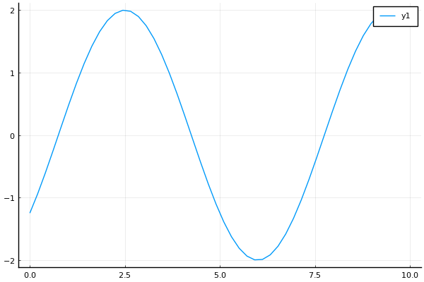
As for the Gaussian noise, we'll create a simple version that simply adds a noise for each data point during sampling.
# File gaussian-noise.jl
export GaussianNoise

struct GaussianNoise <: Sequence
  std
end

GaussianNoise() = GaussianNoise(1.0)

sample(seq::GaussianNoise, t::AbstractVector) = seq.std * randn(length(t))
t = range(0, 10, length=50)
s = GaussianNoise(0.2)
y = sample(s, t)
plot(t, y)Now we can finally combine all of these for an example:
Let's use a timeframe of of 12 months of 30 days;
Since we don't have units, we can choose for the start of the year and for each month we add , i.e., December starts at .
An average mean temperature of ;
A sine wave addition
with (temperature differences should be in Kelvin) amplitude;
period of a year ;
peak temperature at noon of 21/June, the Summer solstice for 2022 in the Northern Hemisphere;
A Gaussian noise of standard deviation .
t = range(0, 11, length=12)
seqs = [
  Constant(15.0),
  SineWave(:from_peak, 15.0, 12.0, (6 + 22 / 30)),
  GaussianNoise(0.5),
]
ys = sample.(seqs, Ref(t))
y = sum(ys)
plot(t, y, leg=false)
title!("Average temperature of 2022 in some city")
xticks!(0:11)
xlabel!("Months since 01/Jan/2022")
ylabel!("Temperature (in degrees Celsius)")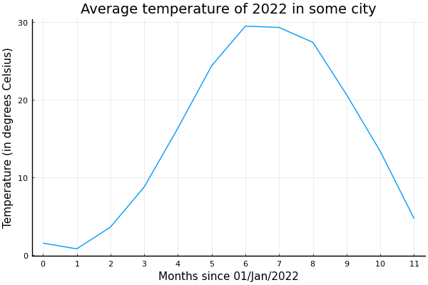
Adding Units using package Unitful
Our example is cool, and our package is working, so we're happy. If you're not happy, you should go and see the Great clown Pagliacci.
Anyway, although cool, we can make it cooler. For that, there is a package called Unitful, which allows the automatic usage and propagation of units in Julia. You should pkg> add Unitful inside the environment, because we should use it on the tests.
After installing, enter julia> using Unitful. You can add units to number by appending them with u"THE-UNIT". For instance,
using Unitful

1u"d", 2u"m" * 3u"m", 2u"hr", 9u"m" / 4u"s"
(1 d, 6 m^2, 2 hr, 2.25 m s^-1)When different units for the same quantity are summed, they are converted to a SI unit. When different units for the same quantity are multiplied or divided, they don't simplify automatically, though.
println("width = ", 30u"cm" + 0.8u"m")
println("area = ", 30u"cm" * 0.8u"m")
println("area = ", uconvert(u"m^2", 30u"cm" * 0.8u"m"))
println("ratio1 = ", 12u"m" / 30u"m")
println("ratio2 = ", 12u"m" / 3000u"cm")
println("ratio2 = ", uconvert(NoUnits, 12u"m" / 3000u"cm"))
width = 1.1 m
area = 24.0 cm m
area = 0.24 m^2
ratio1 = 0.4
ratio2 = 0.004 m cm^-1
ratio2 = 0.4
Most of our code is not restricted by type, so much of it works directly with Unitful. A few things should be changed, though. First, Unitful doesn't accept non-fixed periods, like months or years. So instead of using months, we can change to days and use 30-day months. Additionally, the plot function doesn't allow Unitful by default. So we should add the UnitfulRecipes package as well.
using Unitful, UnitfulRecipes, Plots
month = 30u"d"
t = range(0 * month, 11 * month, length=12)
seqs = [
  Constant(15.0u"°C"),
  SineWave(:from_peak, 15.0u"K", 12month, (6 + 22 / 30) * month),
  GaussianNoise(0.5u"K"),
]
ys = sample.(seqs, Ref(t))
y = uconvert.(u"°C", sum(ys))
plot(t, y, leg=false)
title!("Average temperature of 2022 in some city")
xlabel!("Days since 01/Jan/2022")
ylabel!("Temperature (in degrees Celsius)")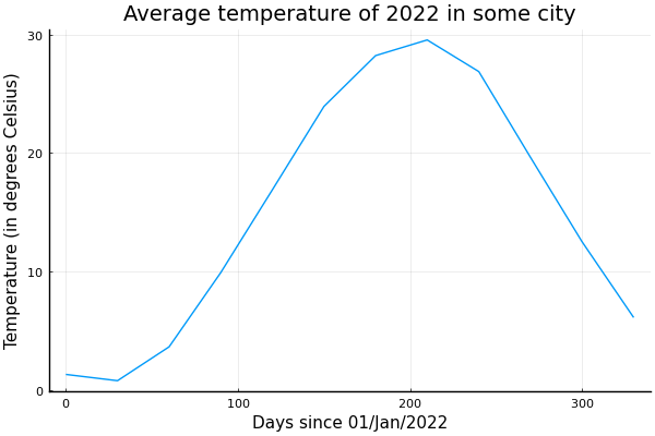
We can refine the interval to see it daily, but notice that the range must change to include the extra time after the beginning of the month. The correct way to define the range with points is to split the interval into equally spaced points, and take the first .
using Unitful, UnitfulRecipes, Plots
n = 360
month = 30u"d"
t = range(0 * month, 12 * month, length=n+1)[1:n]
seqs = [
  Constant(15.0u"°C"),
  SineWave(:from_peak, 15.0u"K", 12month, (6 + 22 / 30) * month),
  GaussianNoise(0.5u"K"),
]
ys = sample.(seqs, Ref(t))
y = uconvert.(u"°C", sum(ys))
plot(t, y, leg=false)
title!("Average temperature of 2022 in some city")
xlabel!("Days since 01/Jan/2022")
ylabel!("Temperature (in degrees Celsius)")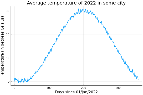
Using units, it's easy to add a new sine wave for daily variations. Let's say for an amplitude of 2 Kelvin with peak at noon. Let's ignore the noise term and focus on shorter period of 3 days starting at the third month.
using Unitful, UnitfulRecipes, Plots
n = 100
month = 30u"d"
t = range(3month, 3month + 3u"d", length=n+1)[1:n]
seqs = [
  Constant(15.0u"°C"),
  SineWave(:from_peak, 15.0u"K", 12month, (6 + 22 / 30) * month),
  SineWave(:from_peak, 2.0u"K", 24u"hr", 12u"hr")
]
ys = sample.(seqs, Ref(t))
y = uconvert.(u"°C", sum(ys))
ticks = range(3month, 3month + 3u"d", step=12u"hr")
plot(t, y, leg=false, xticks=ticks)
title!("Average temperature of 2022 in some city")
xlabel!("Days since 01/Jan/2022")
ylabel!("Temperature (in degrees Celsius)")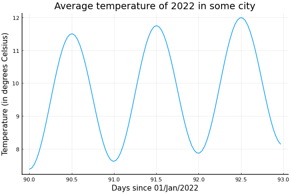
Advanced structures with multiple dispatch
The Unitful usage is only possible because we were generic in many parts of our code by leaving it untyped (which is the same as ::Any). On the other hand, we may benefit from adding types to function arguments to specialize our code. We did that for sample, but now we'll do that for some special functions below.
Now that we have some basic structures, we can start thinking about how they should interact. To obtain a sample of the sum of sequences, we used the sum of the samples. An easier way would be to define a structure to hold the sum of these sequences and do that operation internally. Or better, an operation between sequences. Here's an implementation of that:
# File operation.jl
export OperationOnSequences

struct OperationOnSequences <: Sequence
  seq1
  seq2
  op
end

function sample(seq::OperationOnSequences, t::AbstractVector)
  seq.op.(sample(seq.seq1, t), sample(seq.seq2, t))
end
The OperationOnSequences struct holds two Sequences and an operation op. There's nothing explicitly constraining what that operation is, and that allows us to define whatever we need in the future. The implicit contraint is given by sample. Here, op is applied element-wise to two samples, since Julia allows the . to be used with any function. That means that op must receive two number and return a number.
This is enough to allows us to define the sum of sequences. Test the following:
seqsum = OperationOnSequences(
  SineWave(1.0, 1.0, 0.0),
  SineWave(0.5, 0.25, 0.0),
  +,
)
seqprod = OperationOnSequences(
  SineWave(1.0, 0.2, 0.0),
  Trend(0.5, 2.0),
  *,
)
seqquad = OperationOnSequences(
  Trend(0.25, 4.0),
  Trend(0.8, 2.0),
  *,
)
t = range(0, 1, length=100)
y1 = sample(seqsum, t)
y2 = sample(seqprod, t)
y3 = sample(seqquad, t)
plot(t, y1)
plot!(t, y2)
plot!(t, y3)
Now, we can define directly how the basic operations +, - and * apply to these sequences. In Julia, these operations are just functions - a + b calls +(a, b) - so we just have to define + for our types. That is, we can define Sequence + Sequence to call the constructor to OperationOnSequences.
# File operations.jl
# ...
import Base.+
+(s1::Sequence, s2::Sequence) = OperationOnSequences(s1, s2, +)
s = SineWave(1.0, 2pi, 0.0) + SineWave(0.5, pi, 0.0)
sample(s, 0:pi/4:2pi)9-element Vector{Float64}:
0.0
1.2071067811865475
1.0
0.20710678118654757
0.0
-0.20710678118654746
-0.9999999999999998
-1.2071067811865477
-4.898587196589413e-16We can also automatically transform a Sequence + Number into a Sequence + Constant.
# File operations.jl
# ...
import Base.+
+(s1::Sequence, s2::Sequence) = OperationOnSequences(s1, s2, +)
+(s1::Sequence, x::Number) = OperationOnSequences(s1, Constant(x), +)
s = SineWave(1.0, 2pi, 0.0) + 1
sample(s, 0:pi/2:2pi)5-element Vector{Float64}:
1.0
2.0
1.0000000000000002
0.0
0.9999999999999998Since we're gonna do that for all operations, we can use Metaprogamming to generate the code that we need.
# File operations.jl
# ...
import Base.+, Base.-, Base.*
for op in (:+, :-, :*)
  @eval begin
    $op(s1::Sequence, s2::Sequence) = OperationOnSequences(s1, s2, $op)
    $op(s::Sequence, x::Number) = OperationOnSequences(s, Constant(x), $op)
    $op(x::Number, s::Sequence) = OperationOnSequences(Constant(x), s, $op)
  end
end
Here, first we import the functions +, - and *. Then, op iterates over Symbols storing +, - and *. These are different, note the preceding :. Then, the @eval macro takes the block defined by begin ... end, interpolates the value of op and creates that code for us. This code is equivalent to writing these lines:
+(s1::Sequence, s2::Sequence) = OperationOnSequences(s1, s2, +)
+(s::Sequence, x::Number) = +(s, Constant(x))
+(x::Number, s::Sequence) = +(Constant(x), s)
-(s1::Sequence, s2::Sequence) = OperationOnSequences(s1, s2, -)
-(s::Sequence, x::Number) = -(s, Constant(x))
-(x::Number, s::Sequence) = -(Constant(x), s)
*(s1::Sequence, s2::Sequence) = OperationOnSequences(s1, s2, *)
*(s::Sequence, x::Number) = *(s, Constant(x))
*(x::Number, s::Sequence) = *(Constant(x), s)
Use Metaprogamming sparingly, as the code becomes harder to read.
Here's the same code as before.
seqsum = SineWave(1.0, 1.0, 0.0) + SineWave(0.5, 0.25, 0.0)
seqprod = SineWave(1.0, 0.2, 0.0) * Trend(0.5, 2.0)
seqquad = Trend(0.25, 4.0) * Trend(0.8, 2.0)
t = range(0, 1, length=100)
y1 = sample(seqsum, t)
y2 = sample(seqprod, t)
y3 = sample(seqquad, t)
plot(t, y1)
plot!(t, y2)
plot!(t, y3)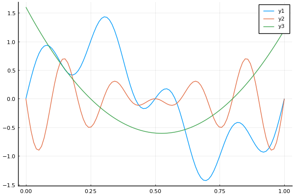
Here's another example:
seq = sum(
  SineWave(1 / (2k + 1), 1 / (2k + 1), 0.0) for k = 0:6
)
t = range(0, 1, length=300)
y = sample(seq, t)
plot(t, y)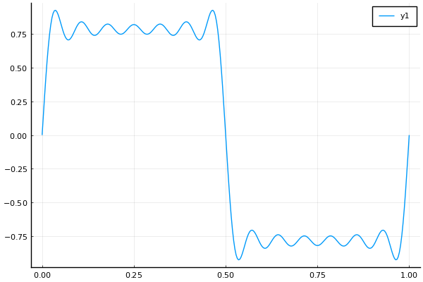
Another useful feature would be the ability to apply functions to sequences. Similarly, we can define a TransformedSequence struct for that:
# File transformation.jl
export TransformedSequence

struct TransformedSequence <: Sequence
  seq
  f
end

function sample(seq::TransformedSequence, t::AbstractVector)
  seq.f.(sample(seq.seq, t))
end

for f in (:exp, :log, :sin, :cos)
  @eval begin
    function Base.$f(s::Sequence)
      TransformedSequence(s, $f)
    end
  end
end
This code is very similar to the previous one. The main difference being that instead of importing the functions, we define the function with the prefix Base. to inform the compiler where it was originally defined. This is an alternative syntax, but for operators, it's a little bit more finnicky.
seqsin = 2 * sin(Trend(0, 2pi))
seqlog = log(1.1 + SineWave(1.0, 1.0, 0.0) + 0.05 * exp(GaussianNoise()))
f(t) = 1 / (1 + exp(-t))
seqf = 5 * TransformedSequence(Trend(0.5, 10), f) - 2
t = range(0, 1, length=100)
y1 = sample(seqsin, t)
y2 = sample(seqlog, t)
y3 = sample(seqf, t)
plot(t, y1)
plot!(t, y2)
plot!(t, y3)
Registration
To finalize this section of the tutorial, let's talk about the registration of our package.
Julia has a community-maintained registry of packages. This registry is accepted as official as part of the Julia ecosystem, and it's the one accessed by the pkg> commands by default. It is not, however, a curated repository. Anyone can register packages in the registry and they're not reviewed before merging.
The exact mechanism by which a package is added to the registry is not simple. Instead, the suggested way of registering a package is by the use of a bot called Registrator.jl. This bot can be installed on your repo on GitHub (for GitLab packages, there is an alternative web interface).
To register our package using the bot, we can perform the following steps.
WARNING: Since this is a package test, probably sending a registration request may be considered bad manners. However, there is nothing strictly forbidding it, as far as I could tell.
After installing the bot, make sure that
versionon theProject.tomlfile is correct and following SemVer.Note that the registry expects your first registration to be a "1", "0.1", or "0.0.1".
Make sure you have committed and uploaded your changes.
On your package GitHub page, open the latest commit.
Leave a message on the commit:
@JuliaRegistrator register.
Best case scenario, that's it. This will create the following course of events:
A comment is posted by
@JuliaRegistratorsaying that all went well and a Pull Request is created at the Registry.The PR at the Registry runs some checks to verify if it will be automatically merged.
It will print a message indicating whether all is fine or what you need to do to address that.
In 3 days the PR is merged, and your package is registered.
If
TagBotis installed (it is in our case), it should trigger the creation of a GitHub tag and release (and with that a Documentation build).
If something went wrong and you need to make fixes, you can just comment @JuliaRegistrator register in the new commit, without modifying the version number.